Tags
To add a footnote in the title of a table or a figure, the following codes may help:
step 1: add \protect \footnotemark in the title
step 2: add \footnotetext{WordsToExplain} neer this title

01 Friday May 2015
Posted in LaTeX
Tags
To add a footnote in the title of a table or a figure, the following codes may help:
step 1: add \protect \footnotemark in the title
step 2: add \footnotetext{WordsToExplain} neer this title
30 Thursday Apr 2015
Posted in LaTeX
Tags
Sometimes section titles include mathematical expressions. The following code can help realize this (taking Euler’s Identity as an example):
\usepackage{hyperref}
\usepackage{bm}
\section{Euler's Identity \texorpdfstring{$\bm{e^{i\pi}+1=0}$}{AnythingHere}}
29 Wednesday Apr 2015
Posted in MATLAB
Tags
Take the implementation of 
Approach I:
s=tf('s');
g1 = (s+1)/(s^2+s+1);
g2 = exp(-s);
g = g1*g2
Approach II:
g=tf([1 1],[1 1 1],'ioDelay',1);
Both the above two approaches give the following result:
Transfer function:
               s + 1
exp(-1*s) * -----------
            s^2 + s + 1
29 Wednesday Apr 2015
Posted in Hardware
Tags
This might be trivial, but sometimes may drive those without much hardware experience crazy 🙂
The wiring method for a DC switching power supply is as follows:
AC input: 110V or 220V, sometimes controlled by a switch
“N” — Null Line;
“L” — Live Line;
“Earth”—Earth Line.
DC output:
“-V” — Negative Output;
“+V” — Positive Output.

Example of a DC switching power supply (S-15-5, Mean Well)
27 Monday Apr 2015
Posted in Statistics
Tags
In k-fold cross-validation, the original sample is randomly partitioned into k equal size subsamples. Of the k subsamples, a single subsample is retained as the validation data for testing the model, and the remaining k − 1 subsamples are used as training data. The cross-validation process is then repeated k times (the folds), with each of the k subsamples used exactly once as the validation data. The k results from the folds can then be averaged (or otherwise combined) to produce a single estimation. The advantage of this method over repeated random sub-sampling (see below) is that all observations are used for both training and validation, and each observation is used for validation exactly once. 10-fold cross-validation is commonly used, but in general k remains an unfixed parameter.
When k = n (the number of observations), the k-fold cross-validation is exactly the leave-one-out cross-validation.
In stratified k-fold cross-validation, the folds are selected so that the mean response value is approximately equal in all the folds. In the case of a dichotomous classification, this means that each fold contains roughly the same proportions of the two types of class labels.
Reference: Wikipedia
24 Friday Apr 2015
Posted in Robotics
Tags
09 Friday May 2014
Posted in Robotics
Tags
The orientation error vector is defined as
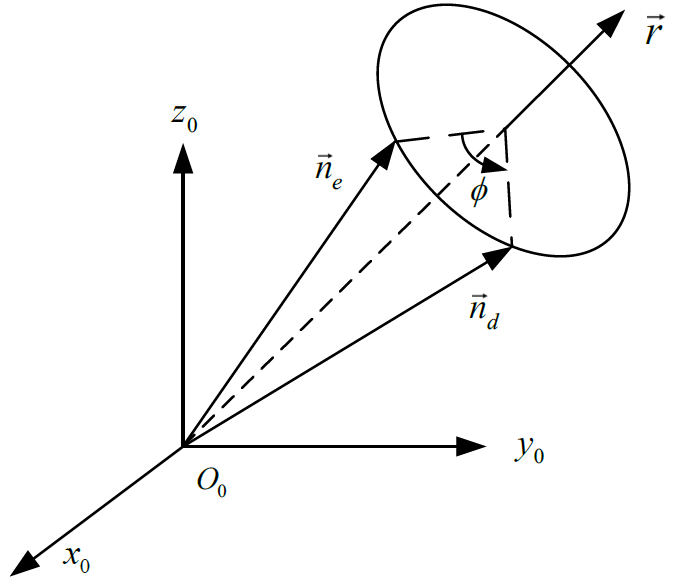
Illustration of the orientation error vector
Reference: Luh, J.Y.S. et al, “Resolved-acceleration control of mechanical manipulators,” IEEE Trans. Automat. Contr., vol.25, no.3, pp.468-474, 1980.
09 Friday May 2014
Posted in Kalman Filter, Linear Systems
Tags
1. Colored process and output noises
2. Non-zero mean process and output noises
3. No output noises
08 Thursday May 2014
Posted in Linear Systems
Tags
Approach I:
Use Kalman Canonical Form Decomposition:
Approach II:
Only check if the modes corresponding to unstable eigenvalues are observable or not. (Since stable modes can always tend to zero asymptotically, we only need to check if the observability of the unstable modes).

 , then check
is equal to n or not.


